Introduction
For those readers who are more mathematically inclined, the treatment below covers the same topics as the Practical Introduction to Factor Analysis up to PCA, but goes more into detail about the matrix operations and formulas involved in factor analysis.
The factor analysis model
Recall that a simple linear regression equation is defined as:
$$y = b_0 + b_1x + \epsilon$$
where \(b_0\) is the intercept and \(b_1\) is the coefficient and \(x\) is an observed predictor. The model for a factor analysis can be thought of as a linear regression where the predictors are unobserved or latent variables. The simple factor analysis model is:
$$y = \tau + \Lambda\eta+ \epsilon$$
where \(\tau\) is the intercept and \(\lambda\) is a regression weight, and \(\epsilon\) is the residual. There are two main differences between the factor analysis model and a linear regression:
- Factor analysis is a multivariate model, meaning that each \(\mathbf{y}\) is actually a vector rather than a single subject, and that each subject has his or her own vector. In a linear regression, you can specify the outcome as a vector, but each subject has his or her own value.
- The predictor \(\eta\) is unobserved or latent whereas in a linear regression the predictors are observed.
Typically we make the assumption that the
- mean of the intercept is zero \(E(\tau)=0\)
- mean of the residual is zero \(E(\epsilon)=0\)
- correlation of the factor with the residual is zero \(Cov(\eta,\epsilon)=0\)
Since factor analysis is a multivariate model, we need to use matrix notation. For a factor analysis with \(q\) factors and \(p\) variables, we would write the same equation as above but instead denote that these are vectors and matrices,
$$ \mathbf{y} = \mathbf{\tau} + \mathbf{\Lambda\eta} + \mathbf{\epsilon} $$
where in the case above \(\mathbf{y}\), \(\mathbf{\tau}\), \(\mathbf{\epsilon}\) are \(p \times 1\) vectors, \(\Lambda\) is a \(p \times q\) matrix and \(\eta\) is a \(q \times 1\) vector. To better understand this notation, let’s spell out a one-factor model with three items. Remember, this is a multivariate model (i.e., multiple outcomes/items) which means the index for \(y_{i}\) is for each item not for a subject.
$$ \begin{pmatrix} y_1 \\ y_2 \\ y_3 \end{pmatrix} = \begin{pmatrix} \tau_{1} \\ \tau_{2} \\ \tau_{3} \end{pmatrix} + \begin{pmatrix} \lambda_{11} \\ \lambda_{21} \\ \lambda_{31} \end{pmatrix} \eta_1 + \begin{pmatrix} \epsilon_1\\ \epsilon_2 \\ \epsilon_3 \end{pmatrix}, $$
note that \(y\), \(\Lambda\) and \(\epsilon\) are \(3 \times 1\) vectors, and \(\eta\) is a scalar. For a two- factor model with three items,
$$ \begin{pmatrix} y_1 \\ y_2 \\ y_3 \end{pmatrix} = \begin{pmatrix} \tau_{1} \\ \tau_{2} \\ \tau_{3} \end{pmatrix} + \begin{pmatrix} \lambda_{11} & \lambda_{12} \\ \lambda_{21} & \lambda_{22} \\ \lambda_{31} & \lambda_{32} \end{pmatrix} \begin{pmatrix} \eta_{1} \\ \eta_{2} \end{pmatrix} + \begin{pmatrix} \epsilon_1\\ \epsilon_2 \\ \epsilon_3 \end{pmatrix}, $$
\(\Lambda\) would become a \(3 \times 2\) matrix, and \(\eta\) becomes a \(2 \times 1\) vector. You could go on and on but the general matrix setup would be the same. If we wanted the average \(\mathbf{y}\) for each item, we can take the expectation (i.e., average),
$$ \begin{eqnarray} \mathbf{\mu_y} = E(\mathbf{y}) &=& E(\mathbf{\tau} + \mathbf{\Lambda} \mathbf{\eta} + \mathbf{\epsilon}) \\ &=& E(\mathbf{\tau} )+E( \mathbf{\Lambda} \mathbf{\eta}) + E(\mathbf{\epsilon}) \\ &=& 0 + E( \mathbf{\Lambda} \mathbf{\eta}) + 0 \\ &=& E( \mathbf{\Lambda} \mathbf{\eta}) \\ &=& \mathbf{\Lambda} E(\mathbf{\eta}) \\ &=& \mathbf{\Lambda} \mathbf{\eta} \end{eqnarray} $$
This is due to the assumptions from above and properties of expectation.
Understanding the covariance structure
Historically, factor analysis is used to answer the question, how much common variance is shared among the items. In order to do that, we would need to find the variance-covariance matrix of the items which we denote \(Cov(\mathbf{y})\) or \(\Sigma(\theta)\). Given what we know from above:
$$ \begin{eqnarray} \Sigma(\theta) = Cov(\mathbf{y}) & = & Cov(\mathbf{\tau} + \mathbf{\Lambda} \mathbf{\eta} + \mathbf{\epsilon}) \\ & = & Var(\mathbf{\tau}) + Cov(\mathbf{\Lambda} \mathbf{\eta}) + Var(\mathbf{\epsilon}) \\ & = & 0 + Cov(\mathbf{\Lambda} \mathbf{\eta}) + Var(\mathbf{\epsilon}) \\ & = & \mathbf{\Lambda} Cov(\mathbf{\eta}) \mathbf{\Lambda}’ + Var(\mathbf{\epsilon}) \\ & = & \mathbf{\Lambda} \Psi \mathbf{\Lambda}’ + \Theta_{\epsilon} \\ \end{eqnarray} $$
This is true due to the assumptions we made above and properties of covariance, such as the fact that the variance of a constant is zero and \(Cov(AB)=A Cov(B) A’\). We have defined new matrices where \(Cov(\mathbf{\eta}) = \Psi\) is the variance-covariance matrix of the factors \(\eta\) and \(Var(\mathbf{\epsilon})=\Theta_{\epsilon}\) is the variance of the residuals. To summarize, here are the terms we have defined so far:
- \(\Lambda\): factor loading matrix (regression coefficients)
- \(\eta\): vector of latent factors (predictor)
- \(\Psi\): variance-covariance matrix of the latent factor (this will be important for rotations later on)
- \(\mathbf{\epsilon}\): vector of residuals (same as residuals in regression)
- \(\Theta_{\epsilon}\): variance-covariance matrix of the residuals (it’s like the Mean Square Error or MSE in ANOVA)
Why do we care so much about the variance-covariance matrix of the outcome? Because the main point of factor analysis is to model the correlation matrix of a set of variables. The basic assumption of factor analysis is that for a collection of observed variables there are a set of underlying factors (smaller than the observed variables, i.e., the \(\eta\)s), that can explain the interrelationships among those variables. These interrelationships start from a Pearson correlation; and since Pearson correlations assume data come from a normal distribution, for the purpose of this seminar we focus only on continuous, linear relationships.
Pearson correlation formula
Before we move on, let’s first remind ourselves of the Pearson product moment correlation for two variables \(X,Y\) which can be defined as:
$$ \rho_{X,Y} = \frac{cov(X,Y)}{\sigma_X \sigma_Y} $$
where \(\sigma_X\) is the standard deviation of \(X\) and \(\sigma_Y\) is the standard deviation of \(Y\).
Example 1
Suppose you know that the correlation of \(\rho_{X,Y}=0.3\), \(\sigma_X=2\), \(\sigma_Y=5\), find the covariance of \(X\) and \(Y\).
Solution:
Rewrite the equation for the correlation as
$$ \begin{eqnarray} cov(X,Y) & = & \rho_{X,Y} \sigma_X \sigma_Y \\ & = & (0.3)(2)(5) = 3 \end{eqnarray} $$
Geometric interpretation of the Pearson correlation
First let’s define the dot product for vectors \(x\) and \(y\):
$$ x \cdotp y = || x || || y || cos(\theta) $$
Let \(\bar{x}\) and \(\bar{y}\) be the means of \(x\) and \(y\) respectively. For a pair of centered variables \(x^{*}=x-\bar{x}\), and \(y^{*}=y-\bar{y}\), the Pearson correlation can be defined as: $$ r = cos(\theta) = \frac{x^{*} \cdotp y^{*}} {|| x^{*} || || y^{*} || } $$
where \( || x^{*} || \) is defined as \(\sqrt{x^{*} \cdotp x^{*}} \), and \( || y^{*} || \) is defined as \(\sqrt{y^{*} \cdotp y^{*}} \). For example, if \(x\) and \(y\) are both three-element vectors:
$$x^{*} \cdotp y^{*} = (x^{*}_1)(y^{*}_1)+(x^{*}_2)(y^{*}_2)+(x^{*}_3)(y^{*}_3)$$
$$|| x^{*} ||= \sqrt{x_1^2+x_2^2+x_3^2}$$
$$|| y^{*} ||= \sqrt{y_1^2+y_2^2+y_3^2}.$$
Example 2
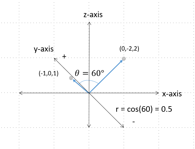
Suppose you have two vectors of data \(x=[1,2,3]’\) and \(y=[2,0,4]’\) and you know that the angle between the vectors is \(60^{\circ}\), find the correlation of the two vectors.
Solution:
We must first center the variables so that \(x^{*}=[-1,0,1]\), and \(y^{*}=[0,-2,2]\). Next we find the magnitude of the centered vectors,
$$ x^{*} \cdotp y^{*} =[(-1)(0)+(0)(-2)+(1)(2)]= 2 $$ $$|| x^{*} || =\sqrt{(-1)^2+(0)^2+(1)^2} = \sqrt{2} $$
$$|| y^{*} || =\sqrt{(0)^2+(-2)^2+(2)^2} = \sqrt{8}$$
$$ \begin{eqnarray} r= cos(\theta) & = & \frac{2} {\sqrt{2}\sqrt{8}} & = & 0.5 \end{eqnarray} $$
Here’s a figure that shows what the vectors and angle look like in a three dimensional space:
Example 3
a) Given that the correlation between two vectors \(x\) and \(y\) is \(r=0.3\), find the angle between the two vectors.
Solution:
We know that \(r = cos(\theta) \) which implies that \( cos^{-1}(r) = \theta \). This means that \( \theta= cos^{-1}(0.3) = 72.54^{\circ} \).
b) Find the angles that correspond to a correlation of -1, 0, and 1. What can you say about the relationship of the angle to positive and negative correlations? Can you make a conjecture about the magnitude of angles as it relates to the magnitude of the correlation?
Solution:
For each of the three correlations \(r=-1,0,1\) we get \( 180^{\circ}, 90^{\circ}\) and \(0\) respectively. This implies that positive correlations range from \(0^{\circ}\) to \(90^{\circ}\) and negative correlations range from \(90^{\circ}\) to \(180^{\circ}\). With a little more observation we can see that
- \( \theta = 0^{\circ}\) implies \(r=1\),
- for \(0^{\circ} < \theta < 90^{\circ}\), the closer the angle is to \(90^{\circ} \) the larger the (positive) correlation,
- \( \theta = 90^{\circ}\) implies \(r=0\) [this is also called orthogonal],
- for \(90^{\circ} < \theta < 180^{\circ}\), the closer the angle is to \(180^{\circ}\), the larger the (negative) correlation, and
- \( \theta = 180^{\circ}\) implies \(r=-1\).
We will use this observation when we learn about orthogonal and oblique rotations in the sections to follow.
Partitioning the variance in factor analysis
Since the goal of factor analysis is to model the interrelationships among items, we focus primarily on the variance rather than the mean. Factor analysis assumes that variance can be partitioned into two types of variance, common and unique
- Common variance is the amount of variance that is shared among a set of items. Items that are highly correlated will share a lot of variance.
- Communality (also called \(h^2\)) is a definition of common variance that ranges between \(0 \) and \(1\). Values closer to 1 suggest that extracted factors explain more of the variance of an individual item.
- Unique variance is any portion of variance that’s not common. There are two types:
- Specific variance: is variance that is specific to a particular variable that is not shared with other items in the analysis but may be shared with other items not in the analysis
- Error variance: comes from errors of measurement, the more reliable the set of items, the less errors there will be (this can assessed by examining reliability using coefficient alpha)
The total variance is the sum of the common and unique variance:
$$ \begin{eqnarray} \mbox{total variance} & = &\mbox{common variance } + \mbox{unique variance} \\ & = &\mbox{common variance } + \mbox{specific variance } + \mbox{error variance} \\ \end{eqnarray} $$
and additionally assuming that the total variance is 1,
$$ \begin{eqnarray} \mbox{communality} + \mbox{unique variance} & = & 1 \\ \mbox{unique variance} & = & 1 – \mbox{communality} \\ & = & 1 – h_i^{2} \end{eqnarray} $$
Let’s get into the communality a little bit more since this appears in the SPSS output and is an essential part of factor extraction. We know that communality is a specific definition of the common variance when the total variance is 1, and its complement is unique variance. Additionally, the sum of communalities across all items is the total variance across all items:
$$ \mbox{total variance} = \sum_{i=1}^{p} h_i^2 $$
Example 4
Consider a special case where the total variance is composed of only the communality. For the SAQ-8, find the total variance.
Solution
If the total variance is composed only of the communality, unique variance is zero which implies the communality of each item \(i\) is 1:
$$ \begin{eqnarray} \mbox{communality}_i + \mbox{unique variance}_i & =& 1\\ \mbox{communality}_i + 0 & = & 1 \\ h^2_i &=& 1 \end{eqnarray} $$
Since there are eight items in the SAQ-8, the total variance is
$$ \mbox{total variance} = \sum_{i=1}^{8} h^2_i = 1 + 1 + 1 + 1 + 1 + 1 + 1 +1 = 8 $$
As we will discuss in the following section, this special case occurs during Principal Components Analysis.
Motivating Example: The SAQ (SPSS Anxiety Questionnaire)
For the remainder of the seminar, we will focus on a hypothetical but real world example of a survey questionnaire which Andy Field terms the SPSS Anxiety Questionnaire. The survey consists of the following 20 questions:
- I dream that Pearson is attacking me with correlation coefficients
- I don’t understand statistics
- I have little experience of computers
- All computers hate me
- I have never been good at mathematics
- My friends are better at statistics than me
- Computers are useful only for playing games
- I did badly at mathematics at school
- People try to tell you that SPSS makes statistics easier to understand but it doesn’t
- I worry that I will cause irreparable damage because of my incompetenece with computers
- Computers have minds of their own and deliberately go wrong whenever I use them
- Computers are out to get me
- I weep openly at the mention of central tendency
- I slip into a coma whenever I see an equation
- SPSS always crashes when I try to use it
- Everybody looks at me when I use SPSS
- I can’t sleep for thoughts of eigen vectors
- I wake up under my duvet thinking that I am trapped under a normal distribtion
- My friends are better at SPSS than I am
- If I’m good at statistics my friends will think I’m a nerd
For simplicity, we will use the so-called “SAQ-8” which consists of the first eight items in the SAQ. Click on the preceding hyperlinks to download the SPSS version of both files.
Let’s explore the data a little bit by using SPSS Analyze – Descriptive Statistics – Descriptives to obtain the following table:
| Correlations | ||||||||
| 1 | 2 | 3 | 4 | 5 | 6 | 7 | 8 | |
| 1 | 1 | |||||||
| 2 | -.099** | 1 | ||||||
| 3 | -.337** | .318** | 1 | |||||
| 4 | .436** | -.112** | -.380** | 1 | ||||
| 5 | .402** | -.119** | -.310** | .401** | 1 | |||
| 6 | .217** | -.074** | -.227** | .278** | .257** | 1 | ||
| 7 | .305** | -.159** | -.382** | .409** | .339** | .514** | 1 | |
| 8 | .331** | -.050* | -.259** | .349** | .269** | .223** | .297** | 1 |
| **. Correlation is significant at the 0.01 level (2-tailed). | ||||||||
| *. Correlation is significant at the 0.05 level (2-tailed). | ||||||||
From this table we can see that most items have some correlation with each other ranging from \(r=-0.382\) for Items 3 and 7 to \(r=.514\) for Items 6 and 7. Due to relatively high correlations among items, this would be a good candidate for factor analysis. Recall that the goal of factor analysis is to model the interrelationships between items with fewer (latent) variables. Let’s talk about various ways to do this in the following section.
Extracting Factors
Now that we understand the factor analysis model and partitioning of variance, we can talk about factor extraction. When extracting factors, we talk about two main parts:
- defining the number of initial factors
- rotating the factors to improve interpretation
The first part, defining initial factors requires making a choice about the type of estimation as well as the number of factors to extract. The second part, rotating factors comes after the number of factors is extracted in order to achieve better interpretability of factors by rotating the factors so we can achieve proximity to what is known as simple structure. There are two approaches to factor extraction which stems from different approaches to variance partitioning: a) principal components analysis and b) common factor analysis.
Principal Components Analysis
Unlike factor analysis, principal components analysis or PCA makes the assumption that there is no unique variance, the total variance is equal to common variance. Recall the formula for variance partitioning,
$$ \begin{eqnarray} \mbox{total variance} & = &\mbox{common variance } + \mbox{unique variance}. \end{eqnarray} $$
If we make the assumption of no unique variance, then
$$ \begin{eqnarray} \mbox{total variance} & = &\mbox{common variance }, \end{eqnarray} $$
and additionally, if we assume total variance is one, then
$$ \begin{eqnarray} \mbox{total variance}_i & = & 1 \\ & = & \mbox{communality}_i \\ & = & h_i^2 \end{eqnarray} $$
Therefore we assume \(h_i^2=1\) for \(i = 1,…,p\) which means that assuming you extracted \(p=q\) components the communality is equal to the total variance.
Quick Poll
Question: Is the communality also equal to the total variance?
(Answer: No, only when \(p=q\). We will see an example of when this is not true later in the seminar.)
Eigenvalues and eigenvectors
The principal components model uses something called spectral decomposition. Essentially what this means is that the correlation matrix \(\mathbf{R}\) can be split up into two symmetric submatrices. Assume that you can obtain a symmetric matrix \(\Delta\) that is a diagonal matrix of eigenvalues and \(\Gamma\) is a matrix of eigenvectors.
$$ \begin{eqnarray} \mathbf{R} & = & (\Gamma \Delta^{1/2})(\Gamma \Delta^{1/2})’ \\ & = & \Gamma \Delta^{1/2} {\Delta^{1/2}}’ {\Gamma}’ \\ & = & \Gamma \Delta \Gamma’ \end{eqnarray} $$
Since the eigenvectors are orthogonal have the unique property that \(\Gamma\Gamma’=\Gamma’\Gamma=I\), or identity.
Eigenvalues (\(\lambda\), not to be confused with the matrix of factor loadings) represent the amount of variance in all of the items. The diagonal elements of \(\Delta\) contain \(\lambda_i\).
$$\Delta = diag(\lambda_1, \lambda_2, \cdots, \lambda_q)$$
Eigenvalues can be thought of as the sum of squared component loadings. They can be positive or negative in theory, but in practice they explain variance which is always positive. The maximum value an eigenvalue can take on in PCA is the variance taken by \(p\) items is also \(p\) since each eigenvalue is restricted to be 1. When eigenvalues are greater than zero, then it’s positive definite (which is a good thing). Since variance cannot be negative, negative eigenvalues imply the model is ill-conditioned. Eigenvalues close to zero imply there is multicollinearity, since all the variance can be taken up by the first component. The eigenvector \(\Gamma\) are otherwise known as factor loadings, which again can be thought of as regression coefficients and represent the correlation of the items with the given component. Think of the eigenvector as a column of weights. So for eight variables there are 8 weights. To obtain the principal component, multiply the weights in an eigenvector by the square root of the eigenvalue.
Example 5
Suppose you have eight items and run a PCA. Assuming that \(\lambda_i \ge 0\), what is the minimum amount of variance that can explained by each PCA component? What is the maximum amount of variance that can be explained by a single PCA component?
Solution
The minimum amount of variance explained by each component in the PCA solution occurs when you extract 8 components, each with an eigenvalue of 1. The maximum amount of variance explained by a single component can be achieved if you extract eight components but only the first component has an eigenvalue of 8 and the others have an eigenvalue of 0. This is a special case where the first component explains \(100\%\) of the total variance.
Components
Given that PCA is principal components analysis, let’s first understand what components are. The goal of a PCA is to replicate the correlation matrix using a set of components that are fewer in number and linear combinations of the original set of items. The components of the PCA can be calculated as
$$z = \Gamma \Delta^{1/2},$$
and which means that the components are a product of the eigenvectors and the square root of the eigenvalues. The first component \(z_1\) is a linear combination of the original variables. The sum of squared component loadings represents the amount of variance explained. The second principal component \(z_2\) is obtained from the residual matrix with \(z_1\) removed (or partialled out), and is uncorrelated with \(z_1\). There is the restriction that the eigenvalue for any subsequent component will be smaller than the previous (e.g., \(\lambda_1 > \lambda_2 > \dots > \lambda_p\)). Therefore the first component has the most variance, last component has the least.
PCA makes the crucial assumption that there is as much variance to be analyzed as there are items, assuming the variables are standardized first. Let’s first standardize the variables and then take the variance. In order to do that in SPSS go to Analyze – Descriptive Statistics – Descriptives and check Save standardized values as variables. Recall that the variance of a standard normal variable is 1. Let’s get use Analyze – Descriptive Statistics – Descriptives – Options – Dispersion and check Variance, here’s a modified arrangement of the output for both the standardized and unstandardized variables in the SAQ-8.
| Descriptive Statistics | ||
| Variance | ||
| Original | Zscore | |
| 1 | 0.686 | 1.000 |
| 2 | 0.724 | 1.000 |
| 3 | 1.156 | 1.000 |
| 4 | 0.900 | 1.000 |
| 5 | 0.931 | 1.000 |
| 6 | 1.259 | 1.000 |
| 7 | 1.215 | 1.000 |
| 8 | 0.761 | 1.000 |
| Sum | 7.631 | 8.000 |
Summing down the rows we get a total variance of 7.631 and 8.000 for the original and standardized variables respectively. This will be important later on as we begin running our first PCA in SPSS.
Running a PCA in SPSS
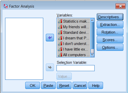
First go to Analyze – Dimension Reduction – Factor. Move all the observed variables over the Variables: box to be analyze.
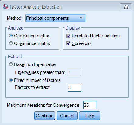
Under Extraction – Method, pick Principal components and make sure to Analyze the Correlation matrix. We also request the Unrotated factor solution and the Scree plot. Under Extract, choose Fixed number of factors, and under Factor to extract enter 8.
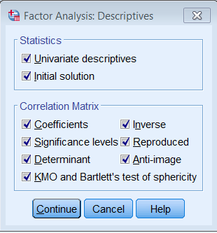
Under Descriptives check all boxes under Statistics and Correlation Matrix.
The equivalent code is shown below:
FACTOR
 /VARIABLES q01 q02 q03 q04 q05 q06 q07 q08
 /MISSING LISTWISE
 /ANALYSIS q01 q02 q03 q04 q05 q06 q07 q08
 /PRINT UNIVARIATE INITIAL CORRELATION SIG DET KMO INV REPR AIC EXTRACTION
 /CRITERIA FACTORS(8) ITERATE(25)
 /EXTRACTION PC
 /ROTATION NOROTATE
 /METHOD=CORRELATION.
Component Matrix
There will be a lot of output from this PCA run but we will highlight only the ones that may seem unfamiliar. Recall that the \(z_{ij}\)s are elements of the table called the Component Matrix. Each of the items down the rows has a loading corresponding to each of the 8 components, and each loading represents the correlation of a particular item with a particular component. For example, Item 1 is correlated .659 with the first component, .136 with the second component and -.398 with the third, and so on.
The square of each loading represents the proportion of variance explained by a particular component. For Item 1, \((0.659)^2=0.434\) or \(43.4%\) of its variance is explained by the first component. Subsequently, \(1.8%\) of the variance in Item 1 is explained by the second component. The total variance explained by both components is thus \(43.4+1.8=45.2%\). As you will see in the next table, if you keep going on adding the squared loadings cumulatively, you find that it sums to 1. This will be true for all items down the row.
| Component Matrixa | ||||||||
| Item | Component | |||||||
| 1 | 2 | 3 | 4 | 5 | 6 | 7 | 8 | |
| 1 | 0.659 | 0.136 | -0.398 | 0.160 | -0.064 | 0.568 | -0.177 | 0.068 |
| 2 | -0.300 | 0.866 | -0.025 | 0.092 | -0.290 | -0.170 | -0.193 | -0.001 |
| 3 | -0.653 | 0.409 | 0.081 | 0.064 | 0.410 | 0.254 | 0.378 | 0.142 |
| 4 | 0.720 | 0.119 | -0.192 | 0.064 | -0.288 | -0.089 | 0.563 | -0.137 |
| 5 | 0.650 | 0.096 | -0.215 | 0.460 | 0.443 | -0.326 | -0.092 | -0.010 |
| 6 | 0.572 | 0.185 | 0.675 | 0.031 | 0.107 | 0.176 | -0.058 | -0.369 |
| 7 | 0.718 | 0.044 | 0.453 | -0.006 | -0.090 | -0.051 | 0.025 | 0.516 |
| 8 | 0.568 | 0.267 | -0.221 | -0.694 | 0.258 | -0.084 | -0.043 | -0.012 |
| Extraction Method: Principal Component Analysis. | ||||||||
| a. 8 components extracted. | ||||||||
Squared Component Loadings
The next table is derived from the Components table. Suppose you took the Components table above and created a table of squared loadings with sums down the rows and columns:
| Item | Squared Loadings for Each Component | ||||||||
| 1 | 2 | 3 | 4 | 5 | 6 | 7 | 8 | Sum | |
| 1 | 0.435 | 0.018 | 0.158 | 0.026 | 0.004 | 0.323 | 0.031 | 0.005 | 1 |
| 2 | 0.090 | 0.751 | 0.001 | 0.009 | 0.084 | 0.029 | 0.037 | 0.000 | 1 |
| 3 | 0.427 | 0.167 | 0.007 | 0.004 | 0.168 | 0.064 | 0.143 | 0.020 | 1 |
| 4 | 0.518 | 0.014 | 0.037 | 0.004 | 0.083 | 0.008 | 0.317 | 0.019 | 1 |
| 5 | 0.422 | 0.009 | 0.046 | 0.212 | 0.196 | 0.106 | 0.008 | 0.000 | 1 |
| 6 | 0.327 | 0.034 | 0.456 | 0.001 | 0.011 | 0.031 | 0.003 | 0.136 | 1 |
| 7 | 0.515 | 0.002 | 0.205 | 0.000 | 0.008 | 0.003 | 0.001 | 0.266 | 1 |
| 8 | 0.323 | 0.071 | 0.049 | 0.481 | 0.066 | 0.007 | 0.002 | 0.000 | 1 |
| Sum | 3.057 | 1.067 | 0.958 | 0.736 | 0.622 | 0.571 | 0.543 | 0.446 | 8 |
Total Variance Explained
Summing down the eight items, you will get the total variance explained by each component. For example, Component 1 is 3.057, or \(3.057/8% = 38.21%\) of the total variance. Note also the last column and the sum down is 8. Compare these results now to the SPSS output Total Variance Explained. Since we extracted eight components, you will see eight rows of eigenvalues.
| Total Variance Explained | ||||||
| Component | Initial Eigenvalues | Extraction Sums of Squared Loadings | ||||
| Total | % of Variance | Cumulative % | Total | % of Variance | Cumulative % | |
| 1 | 3.057 | 38.206 | 38.206 | 3.057 | 38.206 | 38.206 |
| 2 | 1.067 | 13.336 | 51.543 | 1.067 | 13.336 | 51.543 |
| 3 | 0.958 | 11.980 | 63.523 | 0.958 | 11.980 | 63.523 |
| 4 | 0.736 | 9.205 | 72.728 | 0.736 | 9.205 | 72.728 |
| 5 | 0.622 | 7.770 | 80.498 | 0.622 | 7.770 | 80.498 |
| 6 | 0.571 | 7.135 | 87.632 | 0.571 | 7.135 | 87.632 |
| 7 | 0.543 | 6.788 | 94.420 | 0.543 | 6.788 | 94.420 |
| 8 | 0.446 | 5.580 | 100.000 | 0.446 | 5.580 | 100.000 |
| Extraction Method: Principal Component Analysis. | ||||||
Notice that each row in this table is the same as each summed column in the Squared Loadings for Each Component table. Each row in the Total Variance Explained table is the sum of the squared loadings for each component in the PCA. This implies that the sum of the squared loadings in the component matrix of a PCA is the eigenvalue for that item. Suppose a loading of Item \(i\) on Component \(j\) is denoted \(a_{ij}\), this brings us to the eigenvalue equation for the first item as:
$$ \lambda_1 = (z_{11})^{2} + (z_{12})^{2} + \cdots + (z_{1q})^{2} = \sum_{j=1}^{q} (z_{1j})^{2} $$
Additionally, the eigenvalue in a PCA is a measure of the amount of variance attributable to each component. We can sum up all the eigenvalues down the row to calculate the total variance,
$$ \begin{eqnarray} \lambda_1 +\lambda_2 +\lambda_3 +\lambda_4 +\lambda_5 +\lambda_6 +\lambda_7 +\lambda_8 & = & \\ 3.057+1.067+0.958+0.736+0.622+0.571+0.543+0.446 & = & 8 \end{eqnarray} $$
Note that a total variance of 8 matches the descriptives we ran previously to calculate the total variance of our standardized variables. Without defining this explicitly, we already know how to calculate the proportion of total variance. For example for Item 1,
$$\frac{\lambda_{1j}}{\sum_{i=1}^q \lambda_{1j} } = \frac{3.057}{8} = 0.3821 = 38.21\%.$$
The Extraction Sums of Squared Loadings is not always equal to the Initial Eigenvalues. This was only true because we extracted eight components. Here’s the output when you extract two components.
| Total Variance Explained | ||||||
| Component | Initial Eigenvalues | Extraction Sums of Squared Loadings | ||||
| Total | % of Variance | Cumulative % | Total | % of Variance | Cumulative % | |
| 1 | 3.057 | 38.206 | 38.206 | 3.057 | 38.206 | 38.206 |
| 2 | 1.067 | 13.336 | 51.543 | 1.067 | 13.336 | 51.543 |
| 3 | 0.958 | 11.980 | 63.523 | |||
| 4 | 0.736 | 9.205 | 72.728 | |||
| 5 | 0.622 | 7.770 | 80.498 | |||
| 6 | 0.571 | 7.135 | 87.632 | |||
| 7 | 0.543 | 6.788 | 94.420 | |||
| 8 | 0.446 | 5.580 | 100.000 | |||
| Extraction Method: Principal Component Analysis. | ||||||
Notice that the Extracted Sums of Squared Loadings is now simply the first two rows of the Initial Eigenvalues column. The implication here is that using two components, you can explain 51.543% of the variance. Keep in mind that the two component solution is essentially a truncated version of the eight-component PCA, there is nothing inherently different between the two analyses.
Communalities in PCA
Finally, let’s talk about the table of communalities. Recall our assumption that in a PCA, \(h^2\) or the communality is one. PCA is an iterative process which means the solution will change from step to step as it gets closer to the final solution. In this case, the Initial column is what the algorithm starts with as an initial estimate of the communality and this is what it puts into the diagonal of the correlation matrix (which is essentially the correlation matrix itself). The Extraction column is the final solution, which in this case is also one because we extracted eight components.
| Communalities | ||
| Initial | Extraction | |
| 1 | 1.000 | 1.000 |
| 2 | 1.000 | 1.000 |
| 3 | 1.000 | 1.000 |
| 4 | 1.000 | 1.000 |
| 5 | 1.000 | 1.000 |
| 6 | 1.000 | 1.000 |
| 7 | 1.000 | 1.000 |
| 8 | 1.000 | 1.000 |
| Extraction Method: Principal Component Analysis. | ||
The Extraction column may not necessarily be one. Here is a table of communalities when we extract only two components. Notice that the Extraction column is now smaller than one.
| Communalities | ||
| Initial | Extraction | |
| 1 | 1.000 | 0.453 |
| 2 | 1.000 | 0.840 |
| 3 | 1.000 | 0.594 |
| 4 | 1.000 | 0.532 |
| 5 | 1.000 | 0.431 |
| 6 | 1.000 | 0.361 |
| 7 | 1.000 | 0.517 |
| 8 | 1.000 | 0.394 |
| Extraction Method: Principal Component Analysis. | ||
We now have the tools necessary to calculate the Extraction column. The communality is calculated as the sum of the squared loadings up to the \(j\)-th component. Suppose you extract two components and want to calculate the communality for the first item:
$$h^2_1 = (z_{11})^2 + (z_{12})^2 = (0.659)^2 + (0.136)^2 = 0.453$$
Notice that this matches the first row in the Extraction column. An easier way to calculate the communalities is to use the Squared Component Loadings table as shown above. Simply truncate the table to the number of components extracted and sum down the rows.
| Item | Component | ||
| 1 | 2 | Sum | |
| 1 | 0.435 | 0.018 | 0.453 |
| 2 | 0.090 | 0.751 | 0.840 |
| 3 | 0.427 | 0.167 | 0.594 |
| 4 | 0.518 | 0.014 | 0.532 |
| 5 | 0.422 | 0.009 | 0.431 |
| 6 | 0.327 | 0.034 | 0.361 |
| 7 | 0.515 | 0.002 | 0.517 |
| 8 | 0.323 | 0.071 | 0.394 |
| Sum | 3.057 | 1.067 | 4.123 |