Figure 2.1, page 18
get file ="c:\alda\tolerance.sav".
list cases.
      ID    TOL11    TOL12    TOL13    TOL14    TOL15     MALE EXPOSURE
    9.00     2.23     1.79     1.90     2.12     2.66      .00     1.54
   45.00     1.12     1.45     1.45     1.45     1.99     1.00     1.16
  268.00     1.45     1.34     1.99     1.79     1.34     1.00      .90
  314.00     1.22     1.22     1.55     1.12     1.12      .00      .81
  442.00     1.45     1.99     1.45     1.67     1.90      .00     1.13
  514.00     1.34     1.67     2.23     2.12     2.44     1.00      .90
  569.00     1.79     1.90     1.90     1.99     1.99      .00     1.99
  624.00     1.12     1.12     1.22     1.12     1.22     1.00      .98
  723.00     1.22     1.34     1.12     1.00     1.12      .00      .81
  918.00     1.00     1.00     1.22     1.99     1.22      .00     1.21
  949.00     1.99     1.55     1.12     1.45     1.55     1.00      .93
  978.00     1.22     1.34     2.12     3.46     3.32     1.00     1.59
 1105.00     1.34     1.90     1.99     1.90     2.12     1.00     1.38
 1542.00     1.22     1.22     1.99     1.79     2.12      .00     1.44
 1552.00     1.00     1.12     2.23     1.55     1.55      .00     1.04
 1653.00     1.11     1.11     1.34     1.55     2.12      .00     1.25

Number of cases read:  16    Number of cases listed:  16
Creating a person-period data set from a balanced person-level data set and bottom part of Figure 2.1 with person-period data.
* reshaping data into person period data file.
varstocases
 /make tol from tol11 tol12 tol13 tol14 tol15
 /index=measure(5)
 /keep=id exposure male.
compute age=measure+10.
compute time=age-11.
execute.

list cases /var=id age tol male exposure.
      ID      AGE      TOL     MALE EXPOSURE

    9.00    11.00     2.23      .00     1.54
    9.00    12.00     1.79      .00     1.54
    9.00    13.00     1.90      .00     1.54
    9.00    14.00     2.12      .00     1.54
    9.00    15.00     2.66      .00     1.54
   45.00    11.00     1.12     1.00     1.16
   45.00    12.00     1.45     1.00     1.16
   45.00    13.00     1.45     1.00     1.16
   45.00    14.00     1.45     1.00     1.16
   45.00    15.00     1.99     1.00     1.16
 ...........................................
 1653.00    11.00     1.11      .00     1.25
 1653.00    12.00     1.11      .00     1.25
 1653.00    13.00     1.34      .00     1.25
 1653.00    14.00     1.55      .00     1.25
 1653.00    15.00     2.12      .00     1.25

Number of cases read:  80    Number of cases listed:  80
Table 2.1 on page 20, estimated bivariate correlations among tolerance scores.
corr /var=tol11 to tol15.
Figure 2.2 , page 25
formats age tol (f3.0) id (f2.0).
GGRAPH
  /GRAPHDATASET NAME="GraphDataset" VARIABLES= tol age id
  /GRAPHSPEC SOURCE=INLINE INLINETEMPLATE=[ "<setWrapPanels/>"].
BEGIN GPL
SOURCE: s=userSource( id( "GraphDataset" ) )
DATA: tol=col( source(s), name( "tol" ) )
DATA: age=col( source(s), name( "age" ) )
DATA: id=col( source(s), name( "id" ), unit.category() )
GUIDE: text.title( label( "Figure 2.2" ) )
GUIDE: axis( dim( 1 ), label( "age" ) )
GUIDE: axis( dim( 2 ), label( "tol" ) )
GUIDE: axis( dim( 3 ), label( "id" ), opposite() )
SCALE: linear( dim( 1 ), min( 11 ), max( 15 ) )
SCALE: linear( dim( 2 ), min( 0 ), max( 4 ) )
ELEMENT: point( position( summary.mode( age * tol * id ) ) )
END GPL.
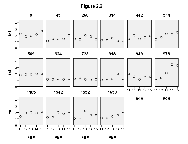
Figure 2.3, page 27
GGRAPH
  /GRAPHDATASET NAME="GraphDataset" VARIABLES= tol age id
  /GRAPHSPEC SOURCE=INLINE INLINETEMPLATE=["<setWrapPanels/>"].
BEGIN GPL
SOURCE: s=userSource( id( "GraphDataset" ) )
DATA: tol=col( source(s), name( "tol" ) )
DATA: age=col( source(s), name( "age" ) )
DATA: id=col( source(s), name( "id" ), unit.category() )
GUIDE: text.title( label( "Figure 2.3" ) )
GUIDE: axis( dim( 1 ), label( "age" ) )
GUIDE: axis( dim( 2 ), label( "tol" ) )
GUIDE: axis( dim( 3 ), label( "id" ), opposite() )
SCALE: linear( dim( 1 ), min( 11 ), max( 15 ) )
SCALE: linear( dim( 2 ), min( 0 ), max( 4 ) )
ELEMENT: line( position( smooth.spline( summary.mode( age * tol * id  ) ) ))
ELEMENT: point( position( summary.mode( age * tol * id ) ) )
END GPL.
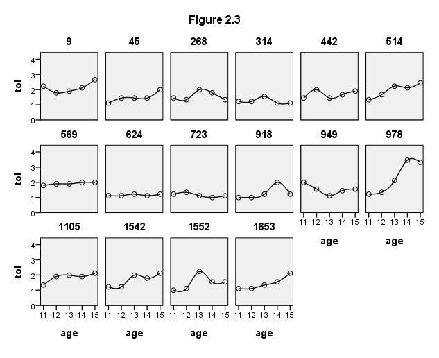
Table 2.2, page 30
Separate regressions for Table 2.2. The first table of Model Summary gives the R-square column. The second table of ANOVA gives the residual variance column which is the Mean Square column for residuals. The last table of Coefficients gives the columns for Initial status and for the rate of change. The last two columns of Table 2.2 can be obtained from the original data set.
sort cases by id.
split file by id.
regress /dep=tol /meth=enter time.
split file off.
Figure 2.4 on page 31, the top part. We can make use of the option from regression to save the parameter estimates to a data file and use this data set for the stem-and-leaf plots. The data set does not contain either R-square or the residual variance for the bottom part of Figure 2.4. So we skip the bottom part now.
get file='C:\alda\tolerance_pp.sav'.
sort cases by id.
split file by id.

REGRESSION
  /DEPENDENT toleranc
  /METHOD=ENTER time
  /OUTFILE=COVB('C:\alda\spsstable2.2.sav') .
get file ='C:\alda\spsstable2.2.sav'.
USE ALL.
COMPUTE filter_$=(rowtype_ = "EST").
FILTER BY filter_$.
EXECUTE .
examine variables=const_ time/plot=stemleaf.
Constant
Constant Stem-and-Leaf Plot
Frequency Stem & Leaf
     1.00        0 .  9
     9.00        1 .  001111234
     6.00        1 .  555789
 Stem width:      1.00
 Each leaf:       1 case(s)
TIME
TIME Stem-and-Leaf Plot
Frequency Stem & Leaf
     2.00       -0 .  59
     1.00       -0 .  3
     3.00        0 .  224
     1.00        0 .  5
     2.00        1 .  14
     3.00        1 .  557
     2.00        2 .  34
     1.00        2 .  6
     1.00 Extremes    (>=.63)
 Stem width:       .10
 Each leaf:       1 case(s)
Figure 2.5, page 32.
formats age tol (f3.0).
GGRAPH
  /GRAPHDATASET NAME="GraphDataset" VARIABLES= tol age id
  /GRAPHSPEC SOURCE=INLINE INLINETEMPLATE=["<setWrapPanels/>"].
BEGIN GPL
SOURCE: s=userSource( id( "GraphDataset" ) )
DATA: tol=col( source(s), name( "tol" ) )
DATA: age=col( source(s), name( "age" ) )
DATA: id=col( source(s), name( "id" ), unit.category() )
GUIDE: text.title( label( "Figure 2.5" ) )
GUIDE: axis( dim( 1 ), label( "age" ) )
GUIDE: axis( dim( 2 ), label( "tol" ) )
GUIDE: axis( dim( 3 ), label( "id" ), opposite() )
SCALE: linear( dim( 1 ), min( 11 ), max( 15 ) )
SCALE: linear( dim( 2 ), min( 0 ), max( 4 ) )
ELEMENT: point( position( age * tol * id ) )
ELEMENT: line( position(smooth.linear( age * tol * id ) ))
END GPL.
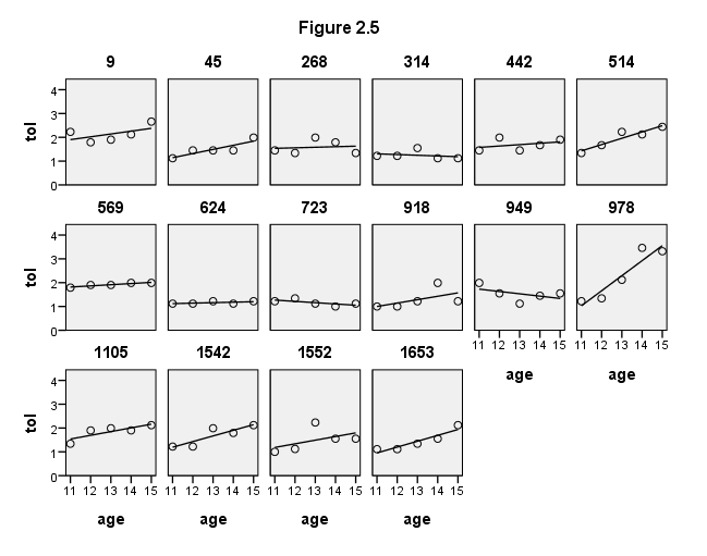
Figure 2.6, page 34, left-hand panel
format tol age (f2.0).
GGRAPH
  /GRAPHDATASET NAME="iGraphDataset" VARIABLES= tol age id
  /GRAPHSPEC SOURCE=INLINE .
BEGIN GPL
SOURCE: s=userSource( id( "iGraphDataset" ) )
DATA: tol=col( source(s), name( "tol" ) )
DATA: age=col( source(s), name( "age" ) )
DATA: id=col( source(s), name( "id" ), unit.category() )
GUIDE: text.title( label( "Figure 2.6, left panel" ) )
GUIDE: axis( dim( 1 ), label( "age" ) )
GUIDE: axis( dim( 2 ), label( "tol" ) )
GUIDE: legend( aesthetic( aesthetic.shape.interior ), null() )
SCALE: linear( dim( 1 ), min( 11 ), max( 15 ) )
SCALE: linear( dim( 2 ), min( 0 ), max( 4 ) )
ELEMENT: line( position( smooth.linear( summary.mode( age * tol ) ) ), shape.interior( id ))
ELEMENT: line( position( smooth.spline( summary.mean( age * tol ) ) ), color( color.red ))
END GPL.
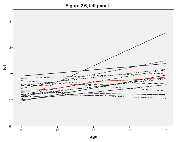
Figure 2.6, page 34, right-hand panel
GGRAPH
  /GRAPHDATASET NAME="GraphDataset" VARIABLES= tol age id
  /GRAPHSPEC SOURCE=INLINE .
BEGIN GPL
SOURCE: s=userSource( id( "GraphDataset" ) )
DATA: tol=col( source(s), name( "tol" ) )
DATA: age=col( source(s), name( "age" ) )
DATA: id=col( source(s), name( "id" ), unit.category() )
GUIDE: text.title( label( "Figure 2.6, right panel" ) )
GUIDE: axis( dim( 1 ), label( "age" ) )
GUIDE: axis( dim( 2 ), label( "tol" ) )
GUIDE: legend( aesthetic( aesthetic.shape.interior ), null() )
SCALE: linear( dim( 1 ), min( 11 ), max( 15 ) )
SCALE: linear( dim( 2 ), min( 0 ), max( 4 ) )
ELEMENT: line( position( smooth.linear( summary.mode( age * tol ) ) ), shape.interior( id ))
ELEMENT: line( position( summary.mean( age * tol ) ), color(color.red) )
END GPL.
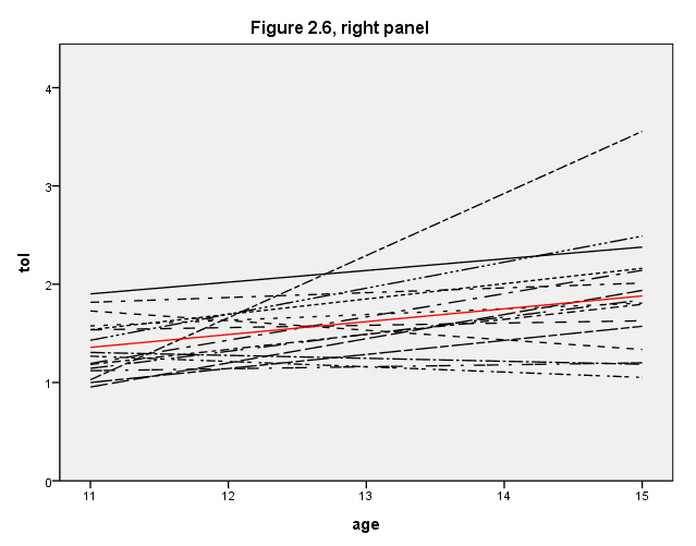
Table 2.3 on page 37. We have created a data set for Figure 2.4 and we can use it here.
get file='C:\alda\spsstable2.2.sav'.
USE ALL.
COMPUTE filter_$=(rowtype_ = "EST").
FILTER BY filter_$.
EXECUTE .
CORRELATIONS
  /VARIABLES=const_ time
  /PRINT=TWOTAIL NOSIG
  /STATISTICS DESCRIPTIVES.
Correlations
Figure 2.7, page 38, upper portion of graph.
compute hiexp = 0.
if (exposure >= 1.145) hiexp = 1 .
execute.

value labels male 0 "male" 1 "female".
GGRAPH
  /GRAPHDATASET NAME="GraphDataset" VARIABLES= tol age id male
  /GRAPHSPEC SOURCE=INLINE
      INLINETEMPLATE=["<setWrapPanels/>"].
BEGIN GPL
SOURCE: s=userSource( id( "GraphDataset" ) )
DATA: tol=col( source(s), name( "tol" ) )
DATA: age=col( source(s), name( "age" ) )
DATA: id=col( source(s), name( "id" ), unit.category() )
DATA: male=col( source(s), name( "male" ), unit.category() )
GUIDE: text.title( label( "Figure 2.7, top row" ) )
GUIDE: axis( dim( 1 ), label( "age" ) )
GUIDE: axis( dim( 2 ), label( "tol" ) )
GUIDE: axis( dim( 3 ), label( "male" ), opposite() )
GUIDE: legend( aesthetic( aesthetic.shape.interior ), null() )
SCALE: linear( dim( 1 ), min( 11 ), max( 15 ) )
SCALE: linear( dim( 2 ), min( 0 ), max( 4 ) )
ELEMENT: line( position( smooth.linear( summary.mode( age * tol * male) ) ), shape.interior( id ))
END GPL.
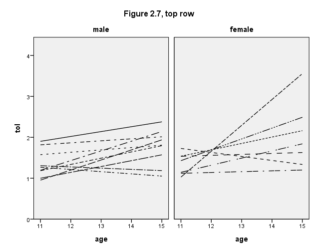
Figure 2.7, page 38, lower portion of graph.
compute hiexp = 0.
if (exposure >= 1.145) hiexp = 1 .
execute.
value labels hiexp 0 "Low exposure" 1 "High exposure".
GGRAPH
  /GRAPHDATASET NAME="GraphDataset" VARIABLES= tol age id hiexp
  /GRAPHSPEC SOURCE=INLINE
      INLINETEMPLATE=["<setWrapPanels/>"].
BEGIN GPL
SOURCE: s=userSource( id( "GraphDataset" ) )
DATA: tol=col( source(s), name( "tol" ) )
DATA: age=col( source(s), name( "age" ) )
DATA: id=col( source(s), name( "id" ), unit.category() )
DATA: hiexp=col( source(s), name( "hiexp" ), unit.category() )
GUIDE: text.title( label( "Figure 2.7, bottom row" ) )
GUIDE: axis( dim( 1 ), label( "age" ) )
GUIDE: axis( dim( 2 ), label( "tol" ) )
GUIDE: axis( dim( 3 ), label( "hiexp" ), opposite() )
GUIDE: legend( aesthetic( aesthetic.shape.interior ), null() )
SCALE: linear( dim( 1 ), min( 11 ), max( 15 ) )
SCALE: linear( dim( 2 ), min( 0 ), max( 4 ) )
ELEMENT: line( position( smooth.linear( summary.mode( age * tol * hiexp) ) ), shape.interior( id ))
END GPL.
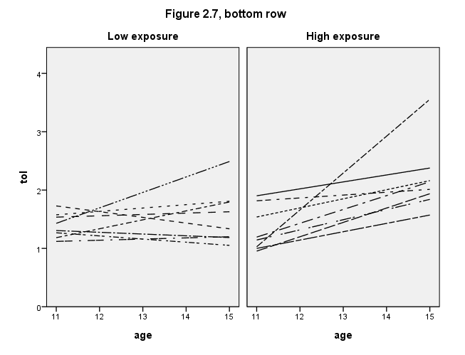
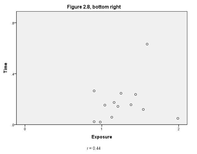
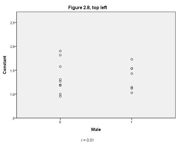
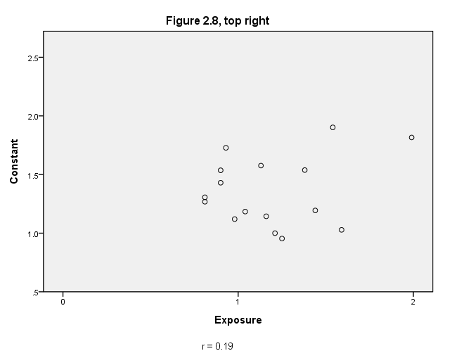
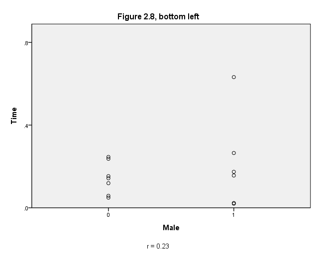
Figure 2.8 on page 40 can be created based on the data set we created for Figure 2.4. The data set is table2.2.sav. We will have to merge it back with the original data set to have all the variables in one data set.
GET
  FILE='C:\alda\table2.2.sav'.

FILTER OFF.
USE ALL.
SELECT IF(rowtype_ = "EST").
EXECUTE .

MATCH FILES /FILE=*
 /RENAME (depvar_ rowtype_ varname_ = d0 d1 d2)
 /FILE='D:aldaspsstolerance.sav'
 /RENAME (tol11 tol12 tol13 tol14 tol15 = d3 d4 d5 d6 d7)
 /BY id
 /DROP= d0 d1 d2 d3 d4 d5 d6 d7.
EXECUTE.
CORRELATIONS
  /VARIABLES=const_ time male exposure.
rename variables CONST_ = const.
formats const (f4.1) male (f1.0).
exe.

GGRAPH
  /GRAPHDATASET NAME="graphdataset" VARIABLES=male const
  /GRAPHSPEC SOURCE=INLINE.
BEGIN GPL
SOURCE: s=userSource(id("graphdataset"))
DATA: male=col(source(s), name("male"), unit.category())
DATA: const=col(source(s), name("const"))
GUIDE: text.title( label( "Figure 2.8, top left" ) )
GUIDE: axis(dim(1), label("Male"))
GUIDE: axis(dim(2), label("Constant"))
GUIDE: text.footnote(label("r = 0.01"))
SCALE: linear(dim(2), min(.5), max(2.5))
ELEMENT: point(position(male*const))
END GPL.
formats exposure (f1.0).
GGRAPH
  /GRAPHDATASET NAME="graphdataset" VARIABLES=exposure const
  /GRAPHSPEC SOURCE=INLINE.
BEGIN GPL
SOURCE: s=userSource(id("graphdataset"))
DATA: exposure=col(source(s), name("exposure"))
DATA: const=col(source(s), name("const"))
GUIDE: text.title( label( "Figure 2.8, top right" ) )
GUIDE: axis(dim(1), label("Exposure"), delta(1))
GUIDE: axis(dim(2), label("Constant"))
GUIDE: text.footnote(label("r = 0.19"))
SCALE: linear(dim(1), min(0), max(2))
SCALE: linear(dim(2), min(.5), max(2.5))
ELEMENT: point(position(exposure*const))
END GPL.
formats time (f3.1).
GGRAPH
  /GRAPHDATASET NAME="graphdataset" VARIABLES=male time
  /GRAPHSPEC SOURCE=INLINE.
BEGIN GPL
SOURCE: s=userSource(id("graphdataset"))
DATA: male=col(source(s), name("male"), unit.category())
DATA: time=col(source(s), name("time"))
GUIDE: text.title( label( "Figure 2.8, bottom left" ) )
GUIDE: axis(dim(1), label("Male"))
GUIDE: axis(dim(2), label("Time"), delta(.4))
GUIDE: text.footnote(label("r = 0.23"))
SCALE: linear(dim(2), min(0), max(.8))
ELEMENT: point(position(male*time))
END GPL.
GGRAPH
  /GRAPHDATASET NAME="graphdataset" VARIABLES=exposure time
  /GRAPHSPEC SOURCE=INLINE.
BEGIN GPL
SOURCE: s=userSource(id("graphdataset"))
DATA: exposure=col(source(s), name("exposure"))
DATA: time=col(source(s), name("time"))
GUIDE: text.title( label( "Figure 2.8, bottom right" ) )
GUIDE: axis(dim(1), label("Exposure"), delta(1))
GUIDE: axis(dim(2), label("Time"), delta(.4))
GUIDE: text.footnote(label("r = 0.44"))
SCALE: linear(dim(1), min(0), max(2))
SCALE: linear(dim(2), min(0), max(.8))
ELEMENT: point(position(exposure*time))
END GPL.