Proc transreg performs transformation regression in which both the outcome and predictor(s) can be transformed and splines can be fit. Splines are piecewise polynomials that can be used to estimate relationships that are difficult to fit with a single function.
In this page, we will walk through an example using some of the most commonly used options of proc transreg. For more information on the options available, see the SAS Online Documentation.
We can begin by creating a dataset with an outcome Y and a predictor X. This example data is generated in the SAS examples for proc transreg.
data a;
  x=-0.000001;
  do i=0 to 199;
    if mod(i,50)=0 then do;
      c=((x/2)-5)**2;
      if i=150 then c=c+5;
      y=c;
      end;
    x=x+0.1;
    y=y-sin(x-c);
	output;
    end;
run;

proc gplot data = a;
  plot y*x;
run;
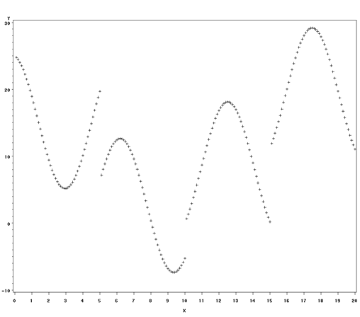
Clearly, there is not a single function relating Y to X. The relationship does not appear random, but it does appear to change with X. Thus it makes sense to try to fit this with splines. We will start with the SAS defaults and then show how you can specify the number of polynomials (pieces) you wish to fit, the degree of the polynomials you wish to fit. Before running the proc transreg, we can see that our data contains four variables:
proc print data = a (obs = 5); run;
Obs       X       I       C          Y

  1    0.10000    0    25.0000    24.7694
  2    0.20000    1    25.0000    24.4427
  3    0.30000    2    25.0000    24.0234
  4    0.40000    3    25.0000    23.5155
  5    0.50000    4    25.0000    22.9241
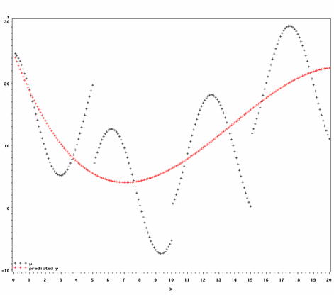
In the proc transreg command, we indicate in the model line that we wish to predict variable y without transformation with identity(y). If we wished to model a transformed version of y (the log or rank of y, for example), we would indicate the transformation here. To predict y, we indicate that we wish to use piecewise polynomial functions of x with pspline(x). There are many other options available that will not be covered in this page. We chose pspline because it is the most commonly used and easy-to-understand option. We also opted to output a dataset, a2, containing predicted values from the model.
proc transreg data=a;
   model identity(y) = pspline(x);
   output out = a2 pprefix = p;
run;

The TRANSREG Procedure

     TRANSREG Univariate Algorithm Iteration History for Identity(Y)
Iteration    Average    Maximum                Criterion
   Number     Change     Change    R-Square       Change    Note
-------------------------------------------------------------------------
        1    0.00000    0.00000     0.46884                 Converged
We can see in the outcome above that the model converged and has an R-squared value of 0.47. Let’s look at the dataset output by proc transreg.
proc print data = a2 (obs = 5); run;
Obs  _TYPE_  _NAME_     Y        TY       pY    Intercept    X_1      X_2

  1  SCORE    ROW1   24.7694  24.7694  24.1144      1      0.10000  0.01000
  2  SCORE    ROW2   24.4427  24.4427  23.4722      1      0.20000  0.04000
  3  SCORE    ROW3   24.0234  24.0234  22.8424      1      0.30000  0.09000
  4  SCORE    ROW4   23.5155  23.5155  22.2249      1      0.40000  0.16000
  5  SCORE    ROW5   22.9241  22.9241  21.6195      1      0.50000  0.25000

  Obs    X_3      TIntercept      TX_1       TX_2       TX_3        X

  1  0.00100         1        0.10000    0.01000    0.00100    0.10000
  2  0.00800         1        0.20000    0.04000    0.00800    0.20000
  3  0.02700         1        0.30000    0.09000    0.02700    0.30000
  4  0.06400         1        0.40000    0.16000    0.06400    0.40000
  5  0.12500         1        0.50000    0.25000    0.12500    0.50000
In addition to adding the predicted values, py, to the dataset, we can see that a new variable, ty, has been added for the "transformed" value of y (since our transformation was the identity, these values are the same as y); three variables (x_1, x_2, x_3) that are the powers of x have been added. Transformations of these three variables and the intercept are also included and indicated with a ‘t‘. We can see that, by default, SAS fits a third-degree polynomial in x to y. We can plot the predicted values to see how closely they match the original data.
legend label=none value=('y' 'predicted y') position=(bottom left inside) mode=share down = 2;
proc gplot data = a2;
   plot (y py)*x / overlay legend = legend;
run;
If we want SAS to fit more than one polynomial, we can indicate that by specifying a number of "knots". A knot is a point at which one polynomial ends and another begins. Similarly, we can indicate the degree of the polynomials to be fit. Generally, as we increase the number of knots or number of degrees, we are able to generate functions that more closely fit the data. This improved fit comes at the cost of estimating more parameters.
Let us look at how we can specify degrees and knots to achieve different types of models.
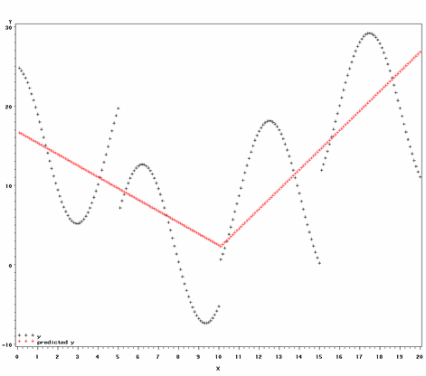
One might believe that x and y are linearly related, but that the slope of the line changes at some point in x. In such a situation, you can fit one one-degree (straight line) polynomial up to the given point in x (the "knot") and another one-degree polynomial from that point on. The proc transreg code for this model and a plot of the results are below.
proc transreg data=a;
   model identity(Y) = pspline(X / nknots=1 degree = 1);
   output out = k1d1 PPREFIX =k1d1;
run;

proc gplot data = k1d1;
   plot (y k1d1y)*x / overlay legend = legend;
run;
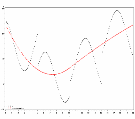
We can improve the fit of the above model by fitting two second-degree polynomials:
proc transreg data=a;
   model identity(Y) = pspline(X / nknots=1 degree = 2);
   output out = k1d2 PPREFIX =k1d2;
run;

proc gplot data = k1d2;
   plot (y k1d2y)*x / overlay legend = legend;
run;
The table below shows how the fit improves with the number of knots and degrees.
| Knots | Degrees | R2 |
| 0 | 1 | 0.10061 |
| 0 | 2 | 0.40720 |
| 0 | 3 | 0.46884 |
| 1 | 1 | 0.47545 |
| 1 | 2 | 0.46467 |
| 2 | 1 | 0.41828 |
| 2 | 2 | 0.51827 |
| 2 | 3 | 0.55391 |
| 3 | 1 | 0.50651 |
| 3 | 2 | 0.53603 |
These are the most basic examples of proc transreg using polynomial splines. SAS offers many examples that employ other options in its online documentation.