The R program for chapter 16.
Table 16.1, p. 420.
First 15 observations only.
print( companies[ 1:15, ])

   type types symbol obsno ror5  de salesgr5  eps5 npm1 pe  payoutr1
 1    1  Chem    dia     1 13.0 0.7     20.2  15.5  7.2  9 0.4263980
 2    1  Chem    dow     2 13.0 0.7     17.2  12.7  7.3  8 0.3806930
 3    1  Chem    stf     3 13.0 0.4     14.5  15.1  7.9  8 0.4067800
 4    1  Chem     dd     4 12.2 0.2     12.9  11.1  5.4  9 0.5681820
 5    1  Chem     uk     5 10.0 0.4     13.6   8.0  6.7  5 0.3245440
 6    1  Chem    psm     6  9.8 0.5     12.1  14.5  3.8  6 0.5108083
 7    1  Chem    gra     7  9.9 0.5     10.2   7.0  4.8 10 0.3789130
 8    1  Chem    hpc     8 10.3 0.3     11.4   8.7  4.5  9 0.4819280
 9    1  Chem    mtc     9  9.5 0.4     13.5   5.9  3.5 11 0.5732480
10    1  Chem    acy    10  9.9 0.4     12.1   4.2  4.6  9 0.4907980
11    1  Chem     cz    11  7.9 0.4     10.8  16.0  3.4  7 0.4891300
12    1  Chem    ald    12  7.3 0.6     15.4   4.9  5.1  7 0.2722770
13    1  Chem    rom    13  7.8 0.4     11.0   3.0  5.6  7 0.3156460
14    1  Chem    rei    14  6.5 0.4     18.7  -3.1  1.3 10 0.3840000
15    2  Heal    hum    15  9.2 2.7     39.8  34.4  5.8 21 0.3908790
Creating the data set companies.std containing the standardized variables.
companies.std <- companies

attach(companies.std)
companies.std$pe.std <- ( pe-mean(pe) ) / stdev(pe)
companies.std$ror5.std <- ( ror5 -mean(ror5 ) ) / stdev(ror5 )
companies.std$de.std <- ( de -mean(de ) ) / stdev(de )
companies.std$salesgr5.std <- ( salesgr5 -mean(salesgr5 ) ) / stdev(salesgr5 )
companies.std$eps5.std <- ( eps5 -mean(eps5 ) ) / stdev(eps5 )
companies.std$npm1.std <- ( npm1 -mean(npm1 ) ) / stdev(npm1 )
companies.std$payoutr1.std <- ( payoutr1 -mean(payoutr1 ) ) / stdev(payoutr1 )

detach(companies.std)
Table 16.2, p. 422.
First 15 observations only.
print( companies.std[1:15, cbind( 1, 2, 3, 13, 14, 15, 16, 17, 12, 11)])

   type types symbol    ror5.std       de.std salesgr5.std    eps5.std
 1    1  Chem    dia  0.96293197 -0.007359609   0.42906692  0.27749331
 2    1  Chem    dow  0.96293197 -0.007359609   0.05047846 -0.05683598
 3    1  Chem    stf  0.96293197 -0.559330289  -0.29025115  0.22973198
 4    1  Chem     dd  0.66059854 -0.927310743  -0.49216499 -0.24788129
 5    1  Chem     uk -0.17081839 -0.559330289  -0.40382769 -0.61803158
 6    1  Chem    psm -0.24640174 -0.375340062  -0.59312191  0.15808999
 7    1  Chem    gra -0.20861007 -0.375340062  -0.83289460 -0.73743489
 8    1  Chem    hpc -0.05744335 -0.743320516  -0.68145922 -0.53444925
 9    1  Chem    mtc -0.35977678 -0.559330289  -0.41644730 -0.86877855
10    1  Chem    acy -0.20861007 -0.559330289  -0.59312191 -1.07176419
11    1  Chem     cz -0.96444364 -0.559330289  -0.75717691  0.33719497
12    1  Chem    ald -1.19119371 -0.191349836  -0.17667461 -0.98818186
13    1  Chem    rom -1.00223532 -0.559330289  -0.73193768 -1.21504817
14    1  Chem    rei -1.49352714 -0.559330289   0.23977269 -1.94340841
15    2  Heal    hum -0.47315182  3.672444925   2.90251150  2.53421603

      npm1.std      pe.std  payoutr1
 1  1.28929042 -0.23732851 0.4263980
 2  1.33381012 -0.44192205 0.3806930
 3  1.60092830 -0.44192205 0.4067800
 4  0.48793588 -0.23732851 0.5681820
 5  1.06669194 -1.05570269 0.3245440
 6 -0.22437927 -0.85110914 0.5108083
 7  0.22081770 -0.03273497 0.3789130
 8  0.08725861 -0.23732851 0.4819280
 9 -0.35793836  0.17185858 0.5732480
10  0.13177830 -0.23732851 0.4907980
11 -0.40245806 -0.64651560 0.4891300
12  0.35437679 -0.64651560 0.2722770
13  0.57697527 -0.64651560 0.3156460
14 -1.33737169 -0.03273497 0.3840000
15  0.66601467  2.21779402 0.3908790
Print out of the first observation to be plotted in the profile diagram in fig. 16.3.
print(companies.std[1, cbind( 13, 14, 15, 16, 17, 12, 18) ] )

  ror5.std       de.std salesgr5.std  eps5.std npm1.std     pe.std
1 0.962932 -0.007359609    0.4290669 0.2774933  1.28929 -0.2373285

  payoutr1.std
1    0.1505715
Creating the transposed data in order to generate the profile diagram.
var1 <- rbind( 1, 2, 3, 4, 5, 6, 7)
values1 <- rbind( 0.962932,  -0.007359609, 0.4290669,
                 0.2774933, 1.28929, -0.2373285, 0.1505715)

graph <- data.frame(values, var1)
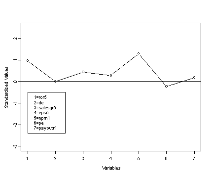
Fig. 16.3, p. 423
Profile diagram of first observation in standardized data set.
plot(graph$var1, graph$values, ylim=c(-3, 2.5), type="b",
     ylab="Standardized Values", xlab="Variables")
abline(h=0)
legend(1, -0.5, c("1=ror5", "2=de", "3=salesgr5",  "4=eps5", "5=npm1",
       "6=pe", "7=payoutr1"))
Print out of the values for observations 16-21 to add to the graph data set.
print(companies.std[15:21, cbind(13, 14, 15, 16, 17, 12, 18)] )

     ror5.std       de.std salesgr5.std   eps5.std   npm1.std     pe.std
15 -0.4731518  3.672444925    2.9025115  2.5342160  0.6660147  2.2177940
16 -0.5865269  0.360620844    1.3881577  1.2327199  1.0666919  2.4223876
17 -0.7754852  0.912591524    2.7636957  1.3640635  0.2653374  1.8086069
18 -0.5487352  0.728601298    0.6688396  1.0416746  0.7550541  1.8086069
19  0.9251403 -0.743320516   -0.1009569  0.3610756  0.6214950  0.7856392
20  1.7943489 -0.007359609   -0.1892942 -0.1881796 -1.2483323 -0.4419221
21  3.0036826 -0.927310743   -0.2271531 -0.1881796 -1.2038126 -0.2373285

   payoutr1.std
15   -0.1347352
16   -1.9789110
17   -0.8403831
18   -0.8380698
19   -0.9651280
20    1.5364365
21    1.3708303
Adding the values for observations 15-21 to the graph data set.
graph$values15 <- rbind(0.4731518, 3.672444925, 2.9025115, 2.5342160, 0.6660147, 2.2177940, 0.1347352)
graph$values16 <- rbind(0.5865269, 0.360620844, 1.3881577, 1.2327199, 1.0666919, 2.4223876, 1.9789110)
graph$values17 <- rbind(0.7754852, 0.912591524, 2.7636957, 1.3640635, 0.2653374, 1.8086069, 0.8403831)
graph$values18 <- rbind(0.5487352, 0.728601298, 0.6688396,  1.0416746, 0.7550541, 1.8086069, 0.8380698)
graph$values19 <- rbind(-0.9251403, -0.743320516, -0.1009569, 0.3610756, 0.6214950, 0.7856392, 0.8380698)
graph$values20 <- rbind(-1.7943489, -0.007359609, -0.1892942, -0.1881796, -1.2483323, -0.4419221, -1.5364365)
graph$values21 <- rbind(-3.0036826, -0.927310743, -0.2271531, -0.1881796, -1.2038126, -0.2373285, -1.3708303)
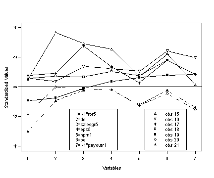
Fig. 16.4, p. 424.
plot(graph$var1, graph$values15, ylim=c(-4, 4), type="b",
     ylab="Standardized Values", xlab="Variables",  pch=2)
abline(h=0)
legend(2.5, -1.5, c("1= -1*ror5", "2=de", "3=salesgr5",  "4=eps5", "5=npm1",
       "6=pe", "7= -1*payoutr1"))
points(graph$var1, graph$values16, type="b", pch=6)
points(graph$var1, graph$values17, type="b", pch=18)
points(graph$var1, graph$values18, type="b", pch=0)
points(graph$var1, graph$values19, type="b", pch=15)
points(graph$var1, graph$values20, type="b", pch=5, lty=4)
points(graph$var1, graph$values21, type="b", pch=17, lty=4)
legend(5.2, -1.5, c("obs 15", "obs 16", "obs 17", "obs 18",  "obs 19", "obs 20", "obs 21"),
       marks=c(2, 6, 18, 0, 15, 5, 17))
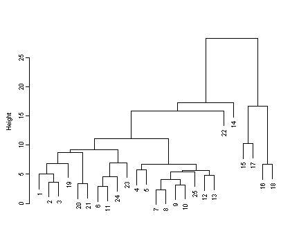
Creating the subset for use in the function agnes.
comp.subset <- companies.std[, cbind(12, 13, 14, 15, 16, 11, 17)]
Fig. 16.9, p. 433.
Not an exact match to the figure in the book but very close.
plot(agnes(comp.subset),which=2)
Creating the subset to be used in the function pam.
attach(companies.std)
comp.subset <- cbind(ror5, de, salesgr5, eps5, npm1, pe, payoutr1)
detach(companies.std)
Table 16.4, p. 435.
These results do not exactly match any of those displayed in the book.
Three clusters.
pam3 <- pam( comp.subset, 3)
print(pam3$clustering)

  1 2 3 4 5 6 7 8 9 10 11 12 13 14 15 16 17 18 19 20 21 22 23 24 25
  1 1 1 1 2 1 2 2 2  2  1  2  2  2  3  3  3  3  1  1  1  1  1  1  2
Table 16.4, p. 435.
Four clusters.
pam4 <- pam( comp.subset, 4)
print(pam4$clustering)

 1 2 3 4 5 6 7 8 9 10 11 12 13 14 15 16 17 18 19 20 21 22 23 24 25
 1 1 1 1 2 3 2 2 2  2  3  2  2  2  4  4  4  4  1  1  1  3  3  3  2